Page /Plans
Use this page to monitor database queries that have a negative impact on system performance, efficiency, or reliability.
Order to go to the /Plans page
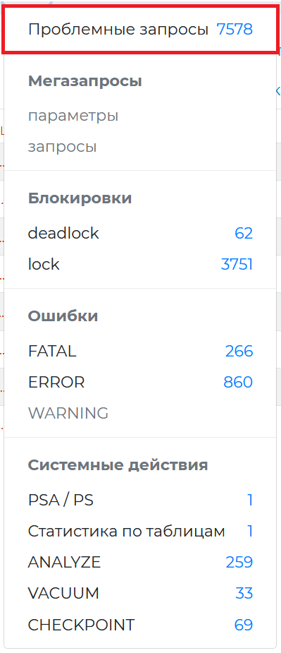
To open this page, click ‘Problematic queries’ link in the burger menu.
Page Control Panel
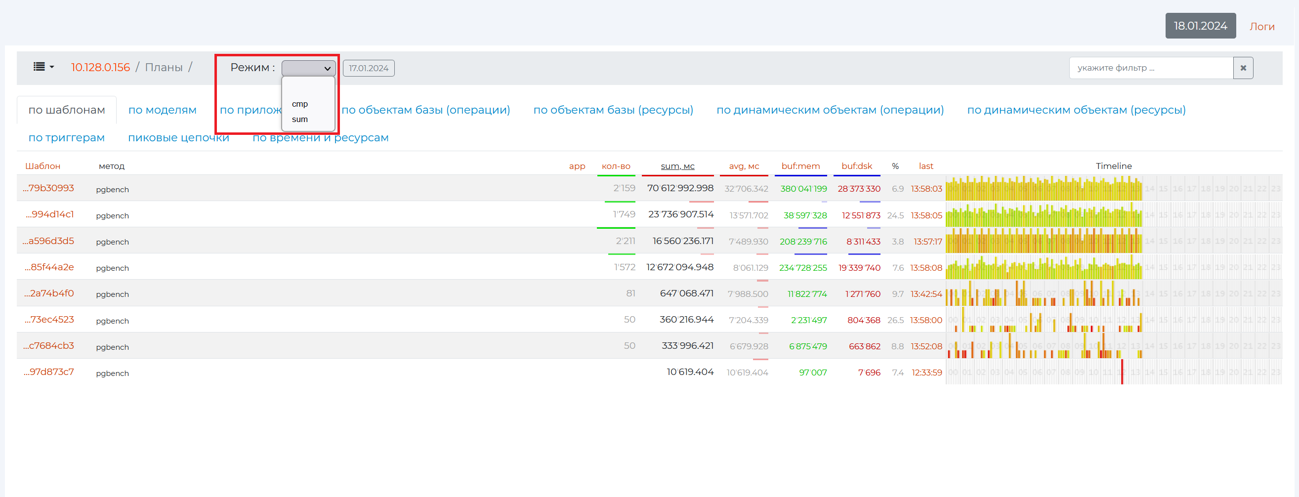
The main page of the section opens. Of the controls that have not been seen before, you can set two modes:
cmp
sum
Let’s take a look at the tabs on this page.
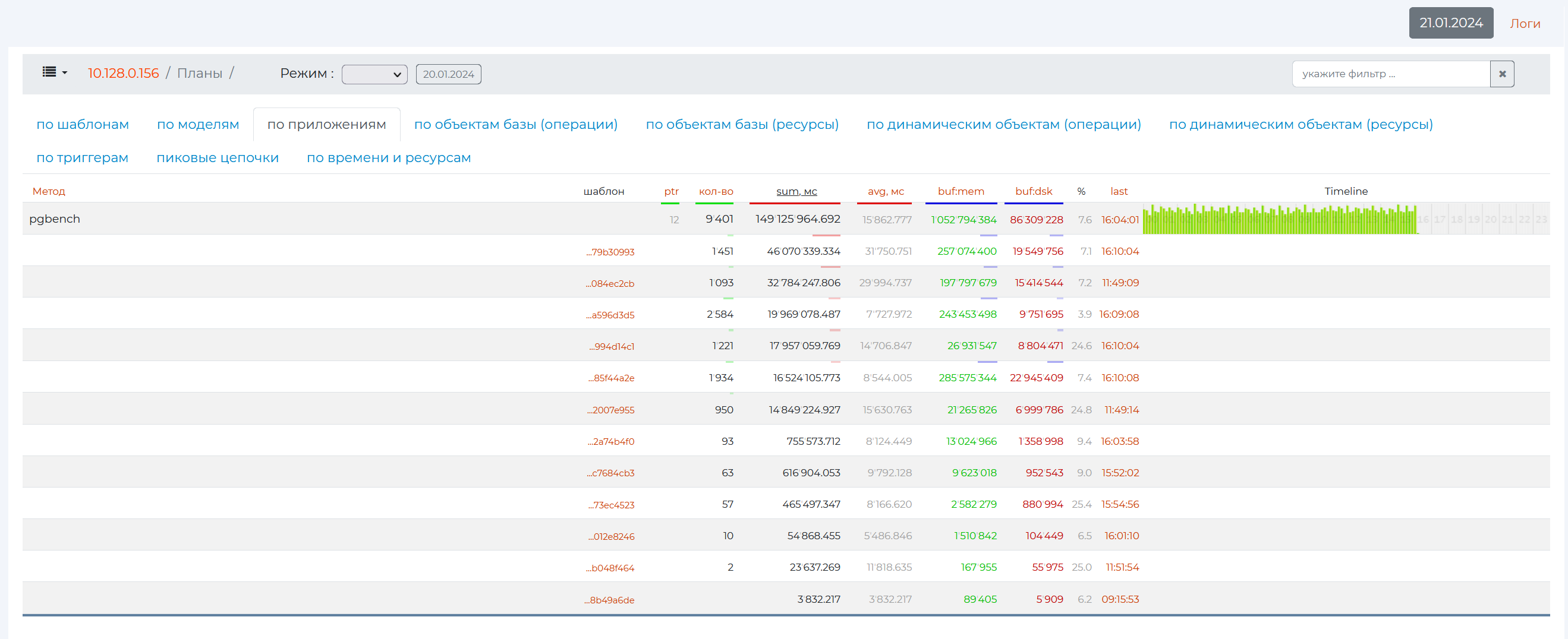
By Patterns tab
This tab contains all the information on queries, sorted by patterns, as well as the main pattern parameters. A pattern is an abbreviated view of the plan, in which the main points of the plan are highlighted with hidden details.

The information is presented in a table containing the following columns:
Pattern is the identification number of the pattern in hexadecimal numeration.
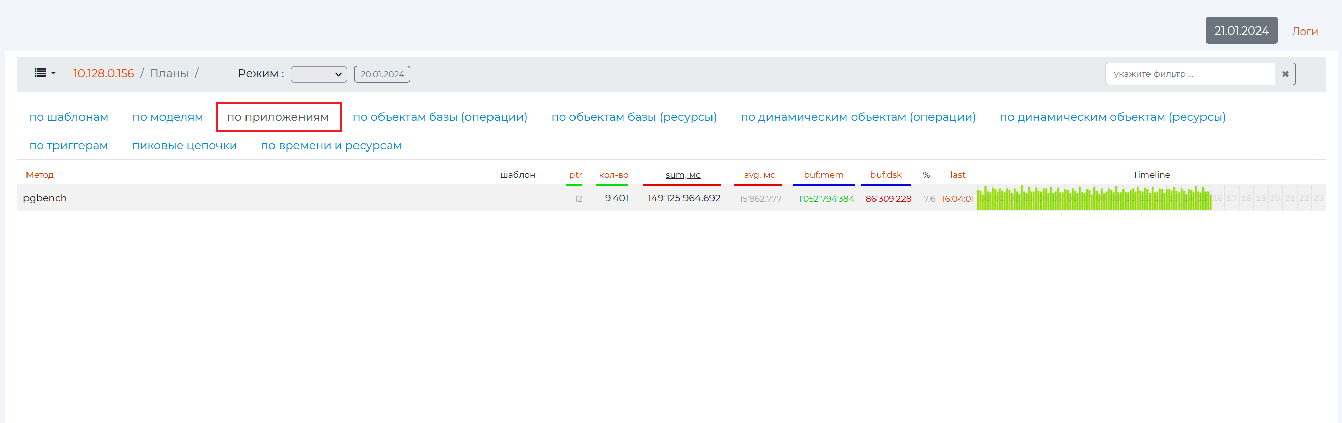
application — PostgreSQL methods that provide analytics on this page. In the screenshot above, in all rows, this method is “pgbench”, a program for running PostgreSQL performance tests. It executes the same sequence of SQL commands over and over again, possibly in multiple concurrent database sessions, and then calculates the average transaction rate (transactions per second).
app — the number of methods used by the pattern, if there are more than one. In this example, all patterns use only one “pgbench” method, so nothing is displayed in the “app” column.
qty — the number of executions of the query that matched the pattern.
sum, mc is the total time it takes to execute queries with this pattern and the time it takes to transfer data. This metric provides information on CPU usage.
avg, mc is the average total time to complete one query.
buf:mem is the total amount of page memory that queries with this pattern “ran” through (not the amount of memory they allocated to themselves).
buf:dsk — shows in data pages (usually one page is 8192 bytes of memory) the amount of memory used by a particular pattern (to understand how much data a single query used, you need to divide the value of this column by the number of queries)
% — shows the percentage of the value of the 8th column from the 7th column.
last is the time at which the last query with this pattern occurred. If you click on the value of this column, you will be taken to the “Request from the archive” page, where a more detailed analysis of this query will be presented.
timeline is a bar graph that shows how the load increases according to a certain pattern over time. The color shows the relative duration of the queries. If the queries are fast, they are green, the slower ones are yellow, and the slowest ones are red. The height of the graph bars is the number of queries in a given period of time. Each strip contains 10 minutes. The entire length of one diagram contains one day, divided into sections by hour.
If you click on the header of any column, the entire table will be sorted by it.
If you click on an empty field of the row, the plan pattern itself will drop out with the names of its nodes.
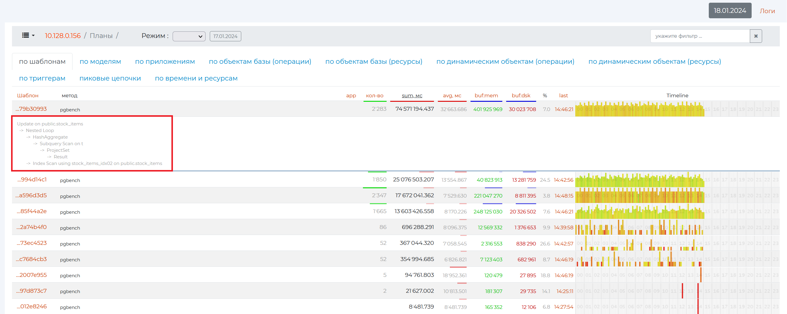
And if you click on the value of the first column, a page with more detailed information on a particular pattern will open.
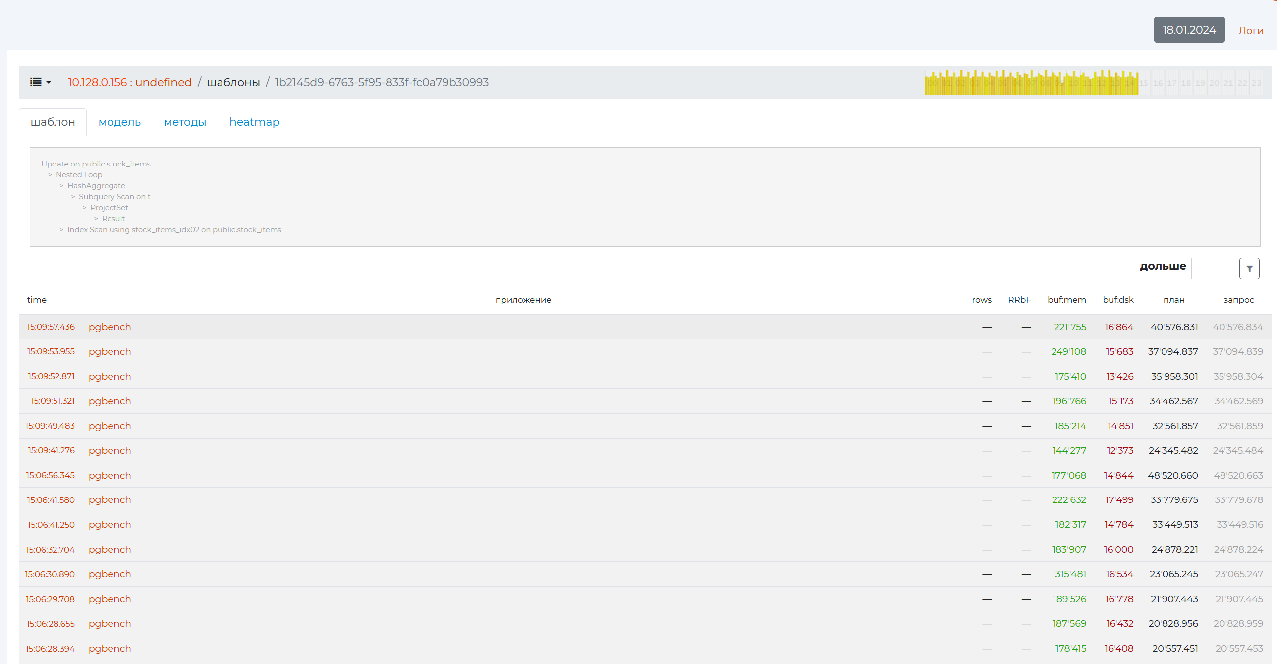
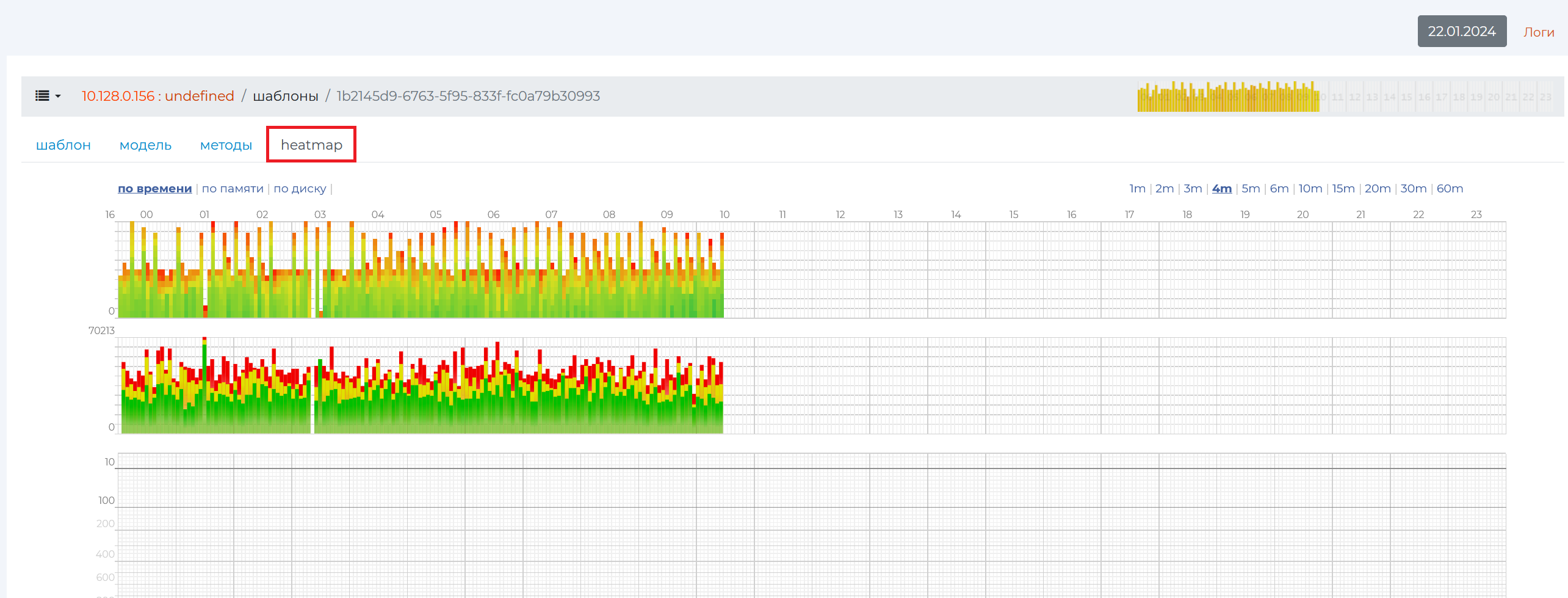
The page has 4 tabs. The Pattern tab at the top shows the same query pattern as the previous page.
At the bottom there is a table with the following columns:
time — time of execution of this query;
applicationы — a method by which metrics were collected;
rows is the number of rows returned;
RRbF — rows removed by filter;
buf:mem is the total amount of memory in pages that this query “ran” through;
buf:dsk is the amount of page memory used by a particular query;
plan — the planned time of query execution — the result of the EXPLAIN command <query_text>;</query_text>
query — Actual Query Execution Time — Result of the EXPLAIN ANALYSE command <query_text>.</query_text>
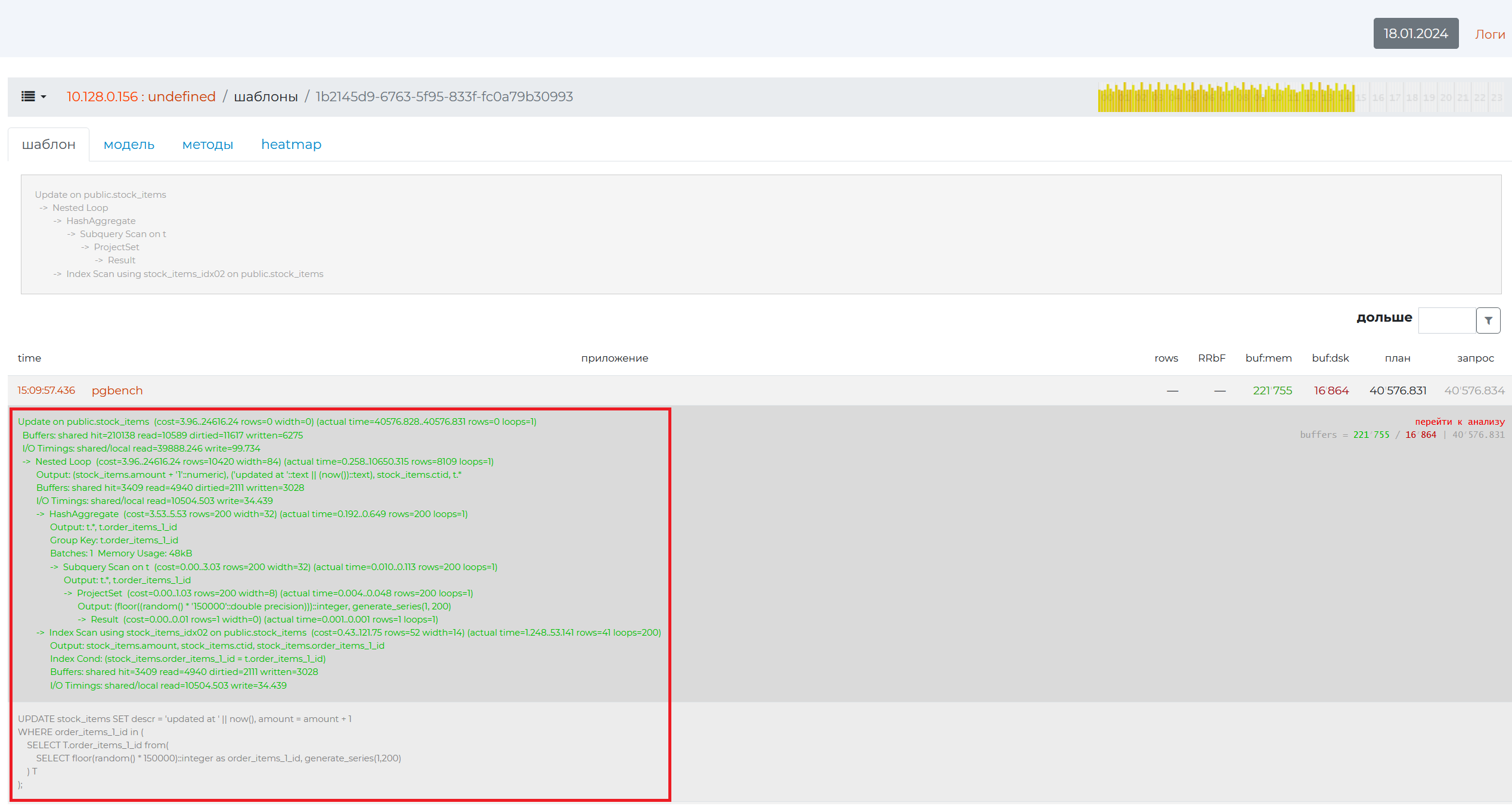
If you click on an empty field of the table row, a detailed query plan will appear (highlighted in green) with details for each node and the text of the query itself (highlighted in gray). All lines contain the text of the same query. Query plans, on the other hand, will differ in the values of the node parameters. All of these plans have a common pattern presented above.
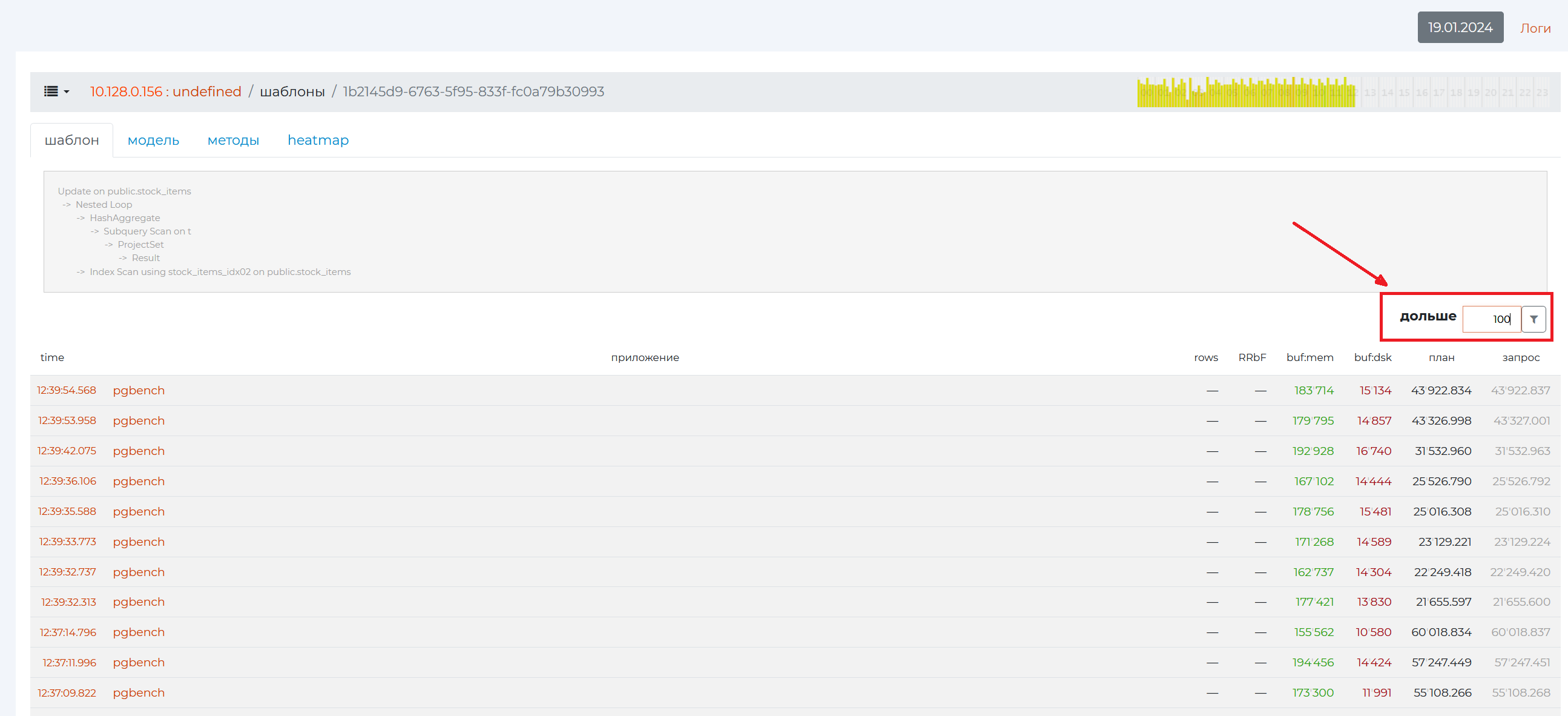
In the filter on the right, you can filter queries by the minimum execution time. Also, the minimum time for logging queries is set in the system configuration. For those queries that do not fall under the filter, statistics will not be collected.
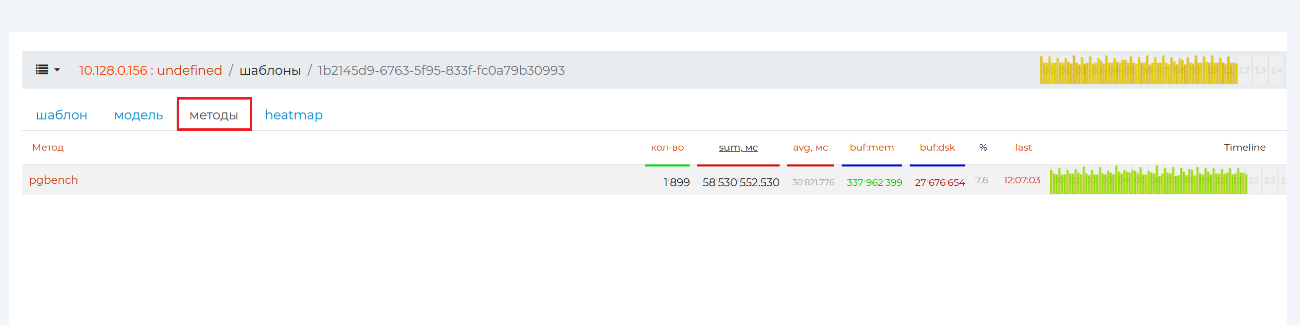
The Methods tab contains the same information as the Pattern tab, only grouped by method instead of specific queries.
At the very top of the “Heatmap” tab is a bar graph showing the distribution of data for this pattern over the past hours. Distribution occurs by time, “by memory” — by cache buffers and by disk. On the horizontal axis there are hours, and on the vertical axis there are strips, each of which contains 10 minutes.
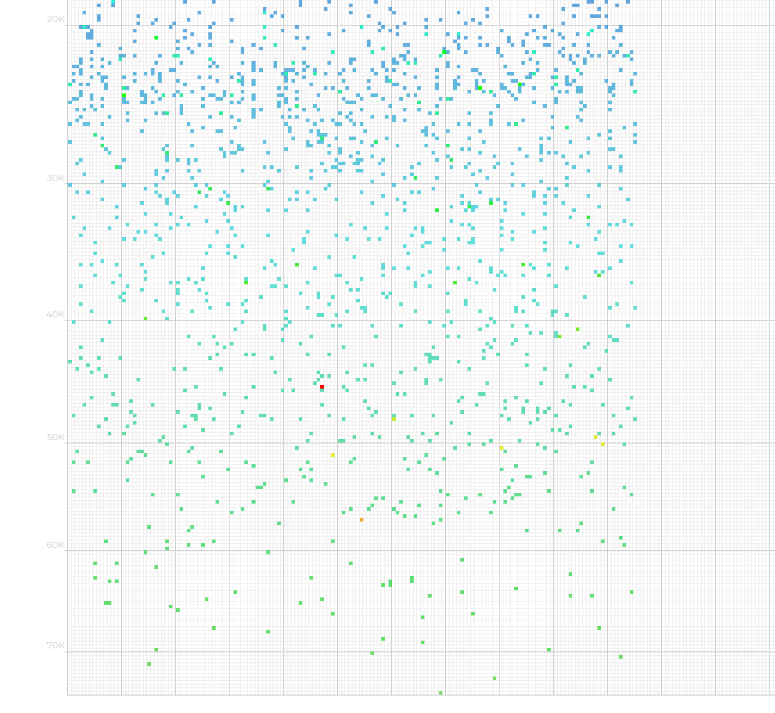
Scrolling to the bottom of this page will bring up a more granular distribution of queries over time.
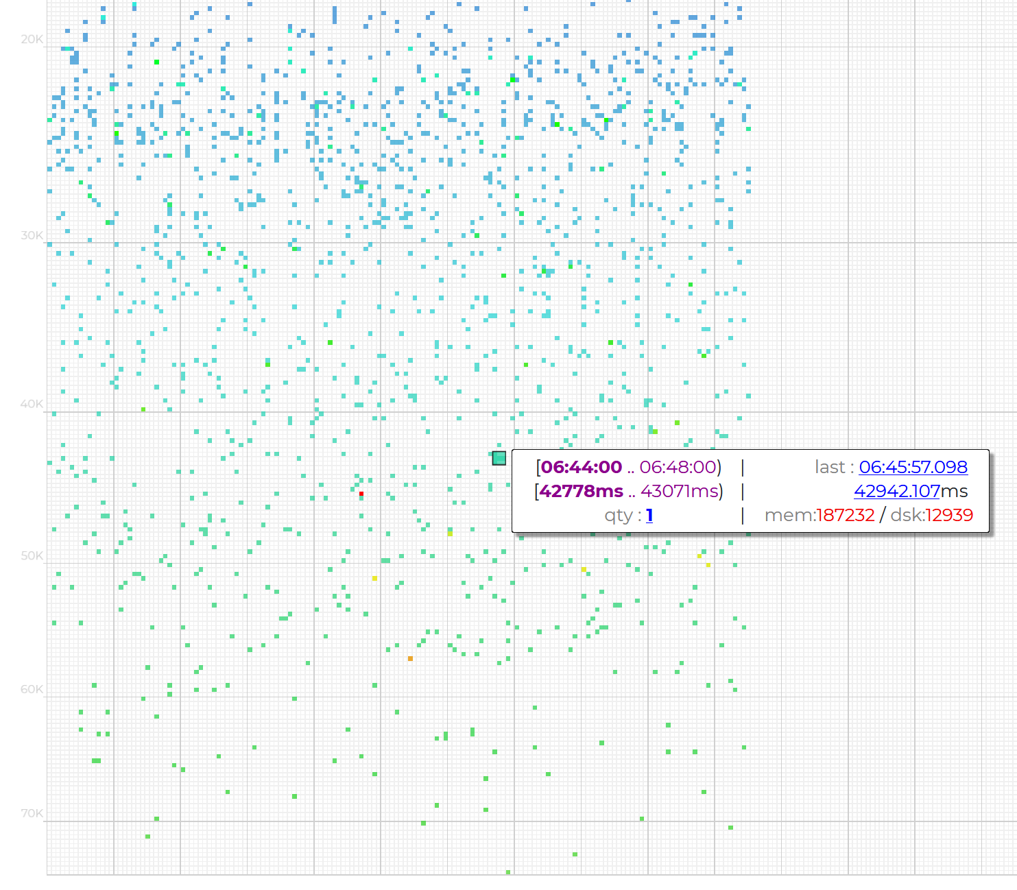
When you hover the mouse cursor over a particular point in the graph, you will see the basic information on these queries from the logs.
By Applications tab
This tab provides the same information as the By Templates tab, but grouped by method.
If you click on the row of this method, patterns for this method will expand.
Here you can also reveal a specific pattern by clicking on the line with its identification number.
When you click on the id of the pattern itself, as well as in the By Patterns tab, the details on it will open.
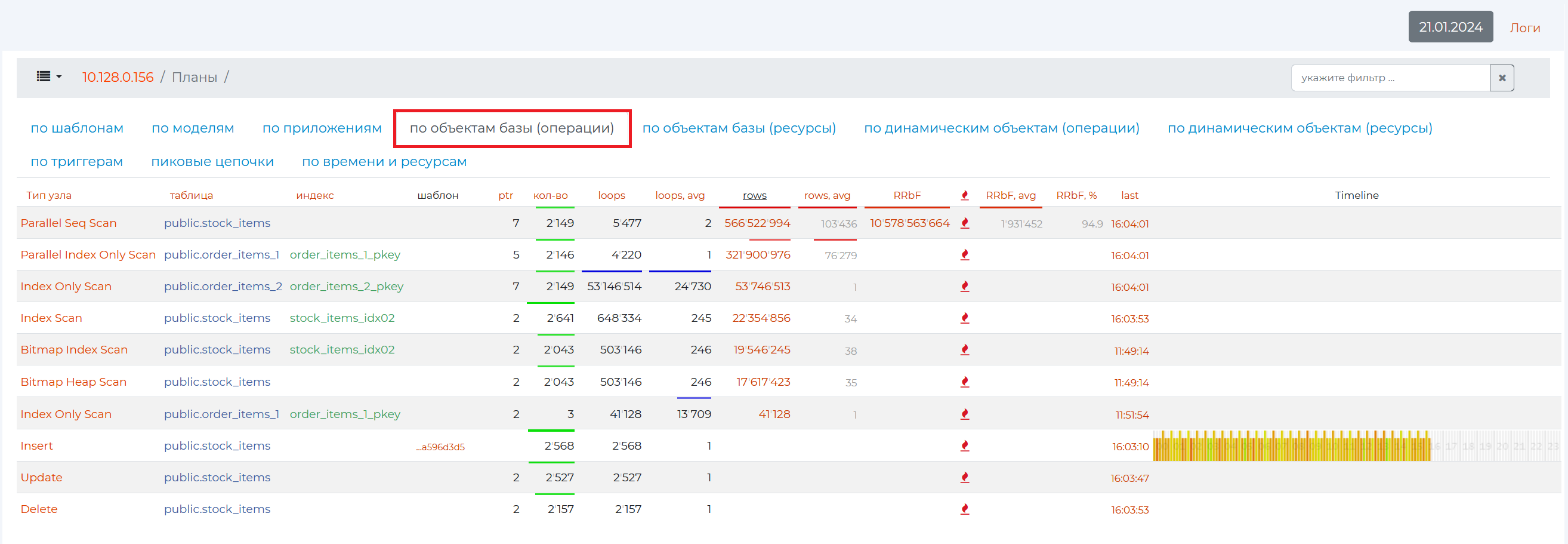
“By database objects (operations) tab”
Databases are tables and their indexes, the names of which are presented in the second (“Table”) and third (“Indexes”) columns of the table in this tab, respectively. Data from databases can be read or written. You can read them simply by iterating through the data using the Seq Scan operation, traversing the index using the Index Scan operation, using bitmaps. The names of the operations of these nodes are presented in the first column.
Clicking on the |node_button| button takes you to the :ref page:/knot <pg_m_узел>.</pg_m_узел>
Thus, the node type is the operation that was performed in a particular query, and the tables and indexes are the database objects that participated in this operation. The remaining columns contain the following data:
Column 4 — when you click on an empty row namespace in this column, the identification numbers of patterns containing such nodes will appear.
Column 5 (PTR) is the number of query patterns with this operation.
Column 6 (qty) is the number of queries with a pattern from the 5th column.
Column 7 (wraparounds) is the number of cycles for this operation.
Column 8 (wraparounds,avg) is the average number of rows returned by a single wraparound with this operation (the result of dividing the value of the 9th column by the value of the 7th column).
Column 9 (rows) is the number of rows that were returned by this operation.
Column 10 (rows, avg) — “rows, average”, the average number of rows returned from the table by one given operation.
Column 11 (RRbF) — “Rows removed by filter”, the number of filtered records in rows (if the value of this column, i.e. the number of rows discarded, is much greater than the number of rows returned — the value of the “rows” column — then this is the result of a not very optimal query, which can cause inconvenience to other users of the server, since it is unreasonable to read so many records to leave such a small percentage later. Using the “Sec Scan” node when the number of records read is also not preferable. It’s about the same with CTEs, as accessing CTE records is much more expensive even than reading from a table with Sec Scan).
Column 12 (RRbF, avg) — “Rows removed by filter, average”, the average number of rows filtered by a given operation.
Column 13 (RRbF, %) — “Rows removed by filter, %”, the number of filtered rows as a percentage of the total number of records in the table.
Column 14 (last) is the time of execution of the last query with such a node.
By clicking on an empty namespace in a row, you can open all patterns with this node in descending order of the number of their repeatability.
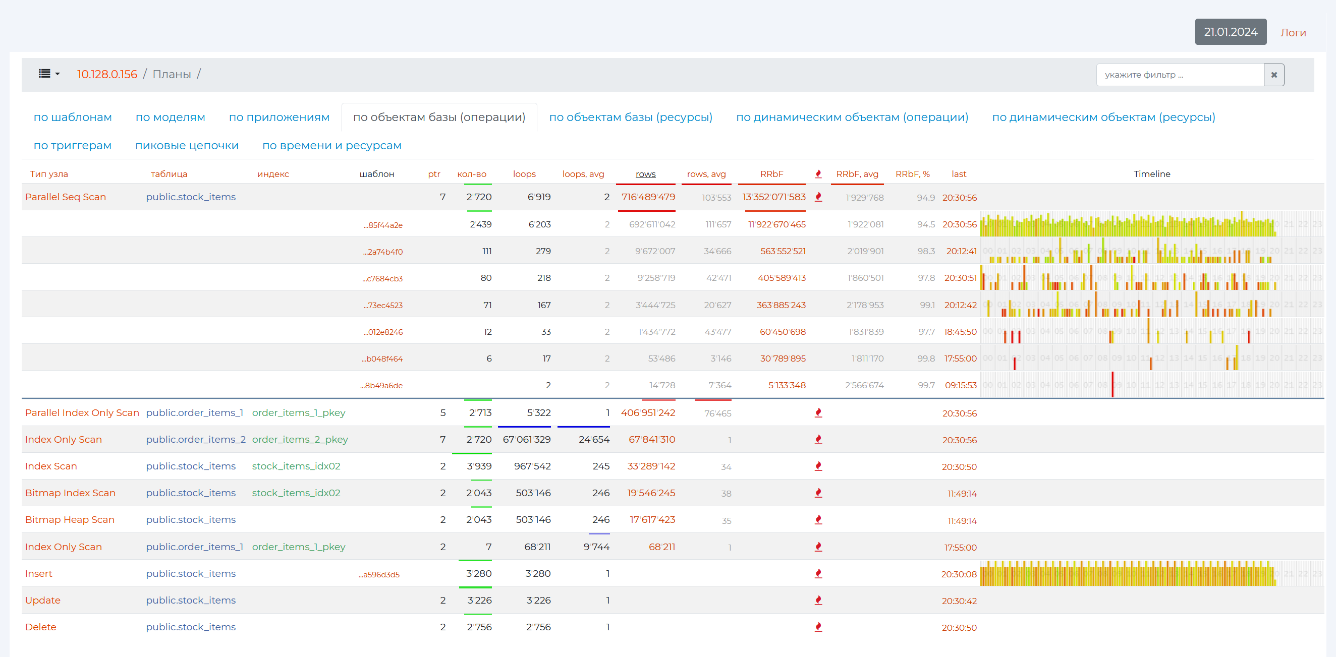
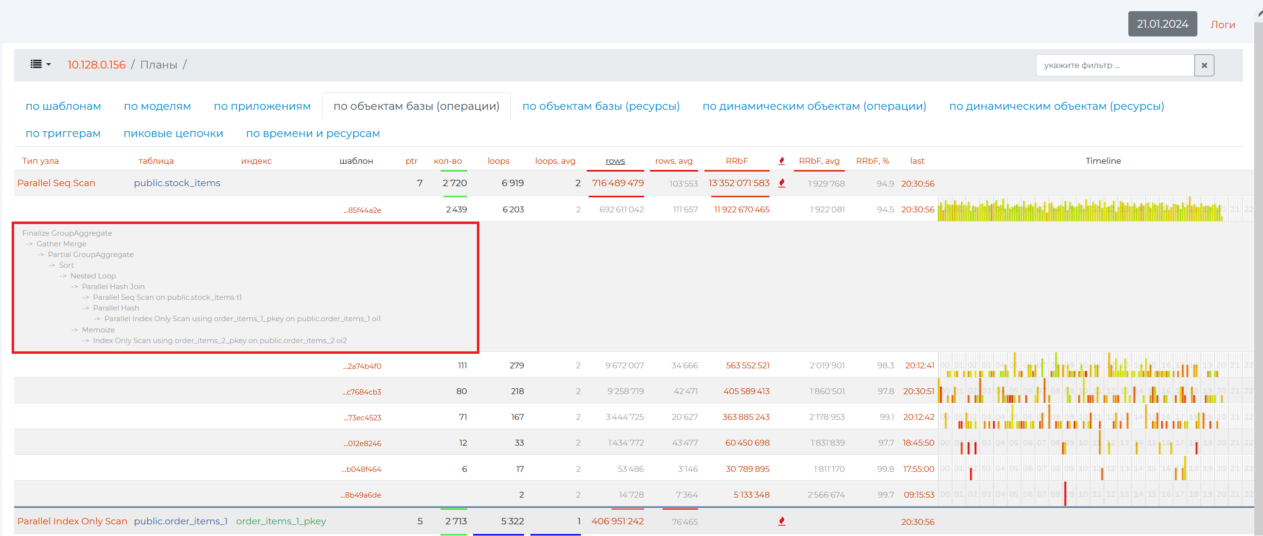
And if you click on the row of a particular pattern, you can look at the entire pattern with all the other nodes.
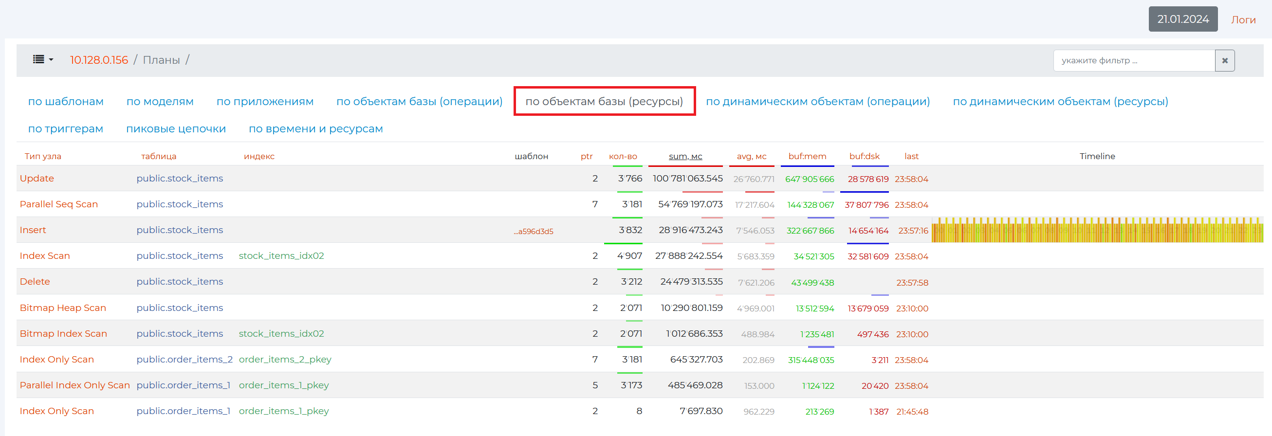
“By database objects (resources) tab”
This tab provides approximately the same information as on the “By database objects (operations)” tab, only with information on the memory resources consumed by this operation (column 7 — sum, mc).
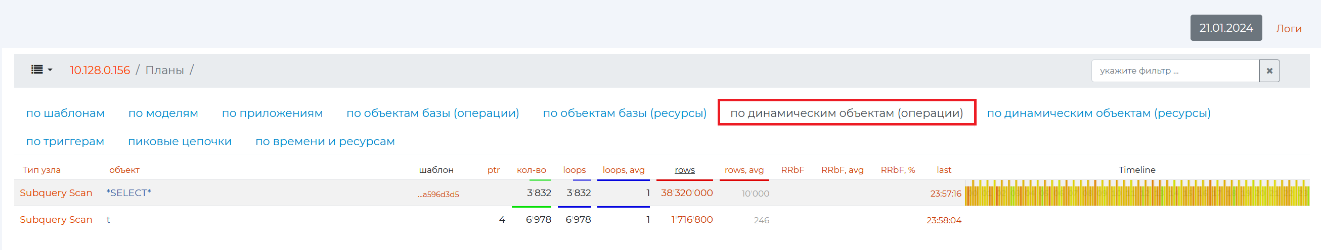
“By dynamic objects (operations) tab”
Sometimes during the execution of a query, dynamic objects arise that are not in the database, but are in the query (various subqueries, Common table expression — CTE, recursive expressions). These dynamic objects are represented in column 2 — “object”.
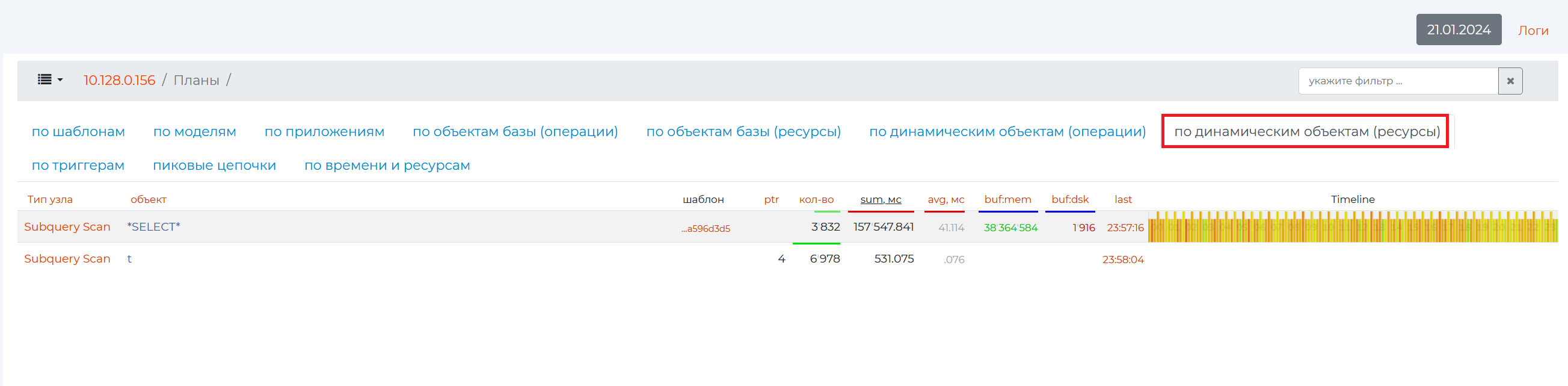
By Dynamic Objects (Resources) tab
Here is the same information as in the previous tab, only from memory.
By Triggers tab
There are two types of triggers:
Custom procedures are special stored procedures that are executed automatically on certain events that occur in the database. These events can be related to changes to tables, such as when data is inserted, updated, or deleted.
Restrictive is a type of trigger that allows you to perform a table-level referential integrity check. They can be used to check the conditions that shall be met before inserting, updating, or deleting data in a table. Restrictive triggers are designed to enforce business rules or constraints that are set for a table.
From the table, you can find out how long it took to complete this trigger, what plans for it happened, and how many times it happened.
Spade Chains Tab
Shows chains of queries for the same pattern that have had little time between executions or that have been executed at the same time. You can see the length of the maximum chain by the number of such consecutive queries. Almost every such chain is a peak CPU usage, so they should be avoided.
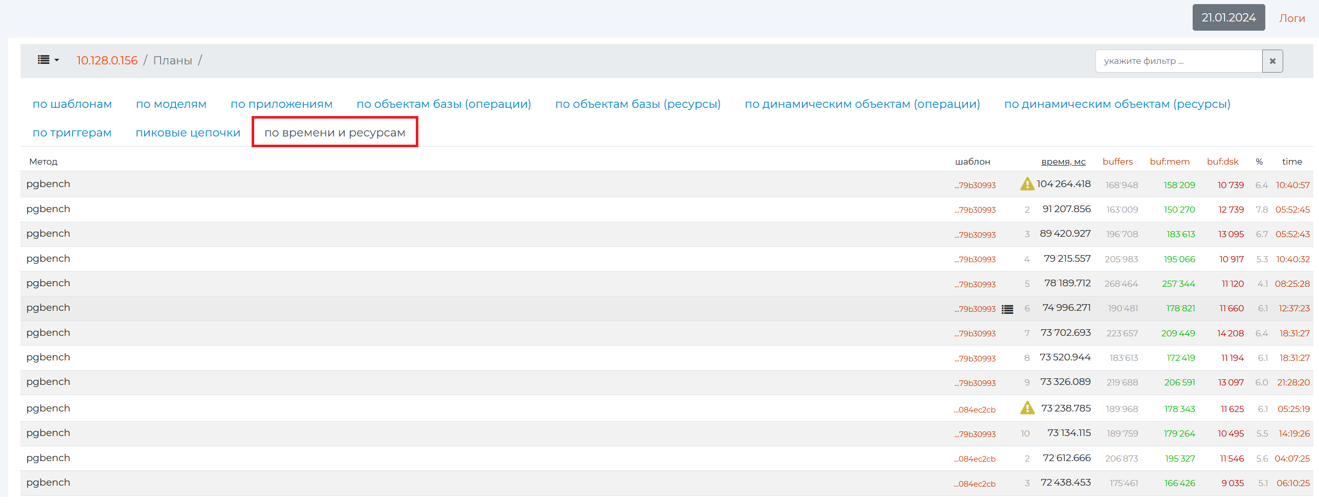
By time and resources tab
This tab shows the same metrics as the By Pattern tab, but the unit of analysis is not the whole plan, but the atomic queries themselves.